ojoThemes Guide

This guide will walk you through the themes and tools available in the ojoThemes package. We’ll start by loading the package (plus tidyverse and ojodb for some test data), then we’ll make some example graphs and tables to show you what’s available.

library(ojothemes)
#> Setting Mac/Linux options...
library(ojodb)
#> Loading required package: dplyr
#> 
#> Attaching package: 'dplyr'
#> The following objects are masked from 'package:stats':
#> 
#>     filter, lag
#> The following objects are masked from 'package:base':
#> 
#>     intersect, setdiff, setequal, union
#> Package 'ojodb' version 2.10.0
library(dplyr)
library(ggplot2)
#> 
#> Attaching package: 'ggplot2'
#> The following objects are masked from 'package:ojothemes':
#> 
#>     geom_bar, geom_col, geom_jitter, geom_line, geom_path, geom_point,
#>     geom_step, geom_text
library(lubridate)
#> 
#> Attaching package: 'lubridate'
#> The following objects are masked from 'package:base':
#> 
#>     date, intersect, setdiff, union
library(gt)

# Test data from OCDC
data <- ojo_tbl(
  schema = "ocdc",
  table = "arrest"
) |>
  filter(
    book_date >= "01-01-2024",
    book_date < "11-01-2024"
  ) |>
  ojo_collect()

Themes for ggplot graphs

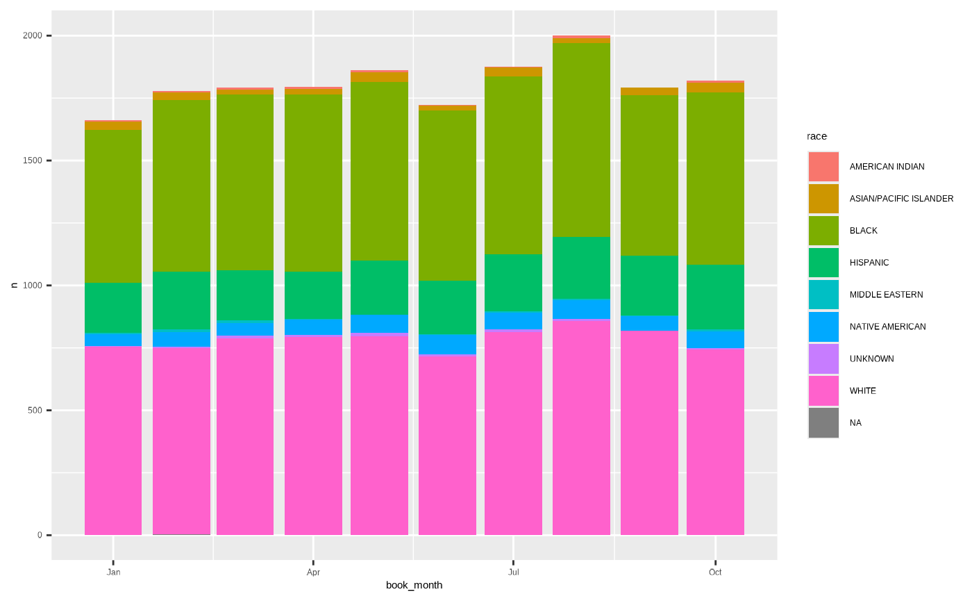
First, let’s see how this data looks on a default ggplot:

p1 <- data |>
  # We'll look at the bookings by race here,
  # and we'll look by month just to make it easier to see.
  count(
    book_month = floor_date(book_date, "months"),
    race
  ) |>
  ggplot(aes(x = book_month, y = n, fill = race)) +
  geom_col()

p1

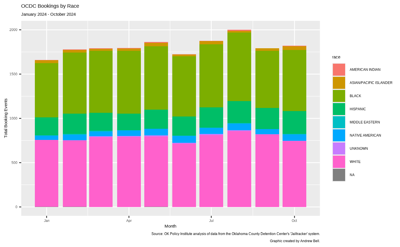
Next, let’s gussy this up with our ojoThemes tools. First, let’s use the ojothemes::ojo_labs() function to easily add a nice caption to the plot:

p1 <- p1 +
  ojo_labs(
    analyst_name = "Andrew Bell",
    source = "ocdc",
    title = "OCDC Bookings by Race",
    subtitle = "January 2024 - October 2024",
    x = "Month",
    y = "Total Booking Events"
  )

p1

This is just a wrapper for the normal ggplot2::labs() function, so we can pass arguments like title, subtitle, x, and y to it. The really neat thing, though, is the new analyst_name and source arguments. These will add a nice little “Graphic created by…” caption crediting the analyst, and a consistently phrased note on where the data came from.

• Right now, you can use "oscn", "ocdc", or "ppb" as the source argument to get a pre-written, consistent source note. However, if you’re working with something not in one of those domains, you can just tell it something to put in there verbatim, e.g. source = "Source: Data Pulled from The National Insitute of My Ass database".

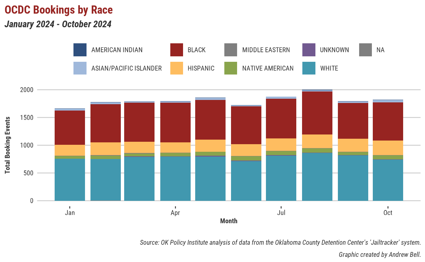
Next, let’s actually apply our themes. There are two ways to do this: the first is to just throw + theme_okpi() onto our ggplot, like so:

p1 + theme_okpi()

This applies not just the theme / fonts, but the color / fill scales as well. If you want just the theme without the scales, you can do p1 + theme_okpi_base().

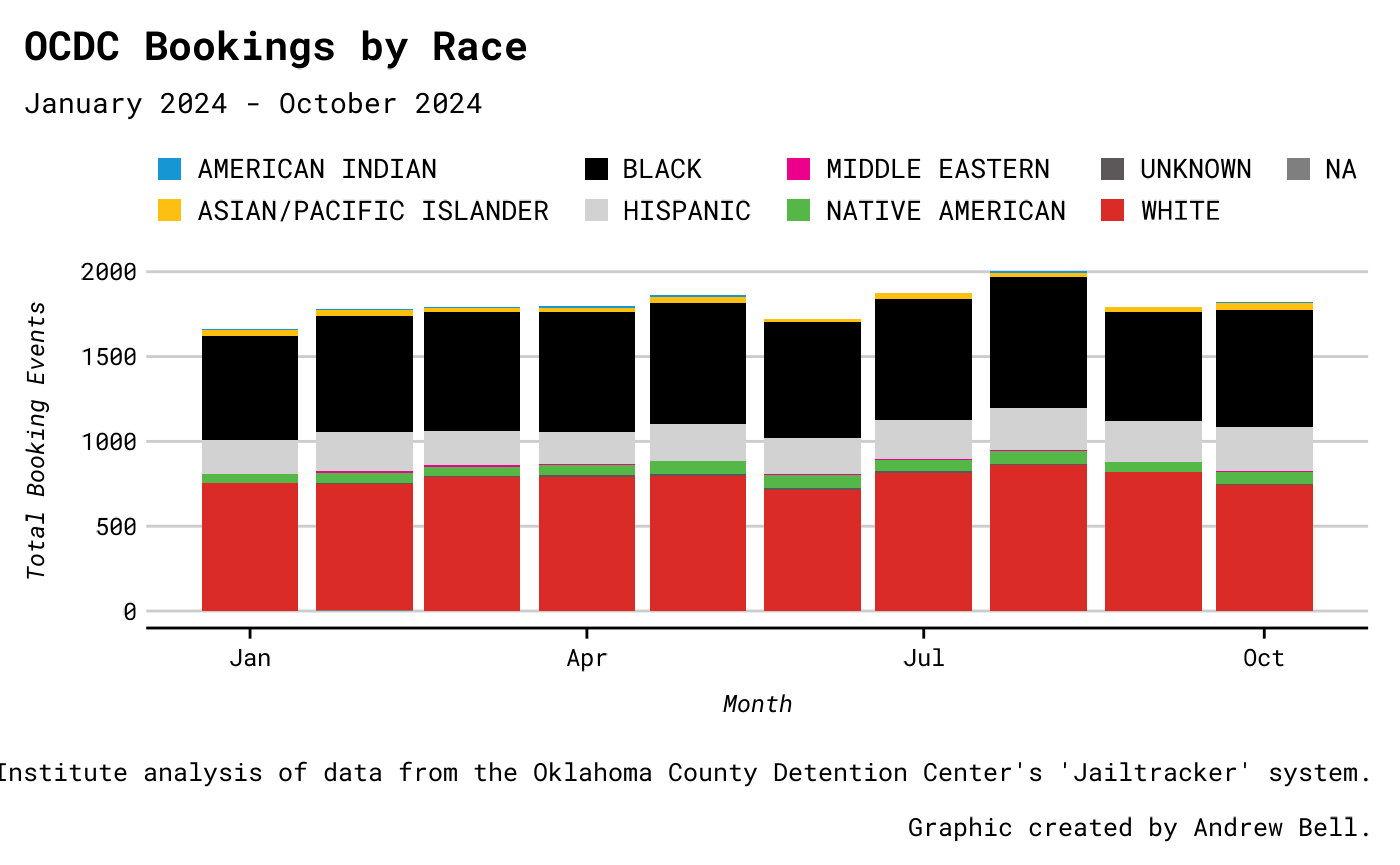
The second way of applying a theme is by using ojothemes::ojo_set_theme(). This is probably going to be the most common way of doing things, since we’re rarely going to want to use multiple themes in the same script / document / etc. Let’s try that same graph in the “ojo” theme this time:

ojo_set_theme(theme = "ojo")

p1

Themes for gt tables

This package also has built in themes for tables made with gt. You can use these by replacing the normal gt() function with one of our themed wrappers (currently gt_okpi() and gt_ojo()). These have built in arguments for customization:

• source and analyst_name (which work just like the ojo_labs() function for ggplots)
• title and subtitle (self explanatory)
• format_cols (a logical that will apply the auto-styling from gt to every column if TRUE)
• font and font_size for making really big / small tables.

Here’s what a normal, unstyled table looks like…

data |>
  count(race) |>
  gt()

race	n
AMERICAN INDIAN	60
ASIAN/PACIFIC ISLANDER	292
BLACK	6931
HISPANIC	2222
MIDDLE EASTERN	53
NATIVE AMERICAN	643
UNKNOWN	70
WHITE	7826
NA	6

…here’s what our gt_okpi() theme does to it…

data |>
  count(race) |>
  gt_okpi(
    title = "OCDC Bookings by Race",
    subtitle = "January 2024 - October 2024",
    source = "ocdc",
    analyst_name = "Andrew Bell",
    format_cols = TRUE
  )

OCDC Bookings by Race
January 2024 - October 2024
race	n
AMERICAN INDIAN	60
ASIAN/PACIFIC ISLANDER	292
BLACK	6,931
HISPANIC	2,222
MIDDLE EASTERN	53
NATIVE AMERICAN	643
UNKNOWN	70
WHITE	7,826
NA	6
Source: OK Policy Institute analysis of data from the Oklahoma County Detention Center's 'Jailtracker' system.
Graphic created by Andrew Bell.

…and finally, here’s gt_ojo():

data |>
  count(race) |>
  gt_ojo(
    title = "OCDC Bookings by Race",
    subtitle = "January 2024 - October 2024",
    source = "ocdc",
    analyst_name = "Andrew Bell",
    format_cols = TRUE
  )

OCDC Bookings by Race
January 2024 - October 2024
race	n
AMERICAN INDIAN	60
ASIAN/PACIFIC ISLANDER	292
BLACK	6,931
HISPANIC	2,222
MIDDLE EASTERN	53
NATIVE AMERICAN	643
UNKNOWN	70
WHITE	7,826
NA	6
Source: OK Policy Institute analysis of data from the Oklahoma County Detention Center's 'Jailtracker' system.
Graphic created by Andrew Bell.