Pulling court data with ojodb

#> <PqConnection> ojodb@34.122.10.67:5432

Intro: The OJO database

Many of our projects and requests involve pulling court data from our OJO database. There are a few other organizations and authorities who have collected this type of data in Oklahoma, but we’re somewhat unique in the amount of data we have and the tools we’ve developed to pull and analyze it.

Our court data comes from two sources:

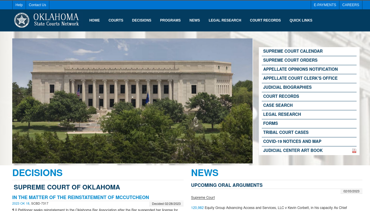
The Oklahoma State Court Network website, the official record for the most populous and organized counties in the state, and
The On Demand Court Records website, an alternate official record used by the less populous counties.

We scrape the data posted on these websites each day, and store the contents in our database.

Having the data scraped and wrangled like this lets us answer questions that are harder to get a handle on otherwise. For example, legislators and stakeholders will often want to know things like “How many felonies were filed from 2016-2022?”, or “How did eviction filings change during COVID, or as a result of X policy change?” It can be shockingly hard to answer even basic questions like that, even for government officials, and that’s where our database comes in!

To get an idea of how to use the database to answer these kinds of questions, this vignette will walk through all the steps for a hypothetical research question.

Research Question:

How many misdemeanor cases involving drugs were filed in Oklahoma and Tulsa county in each month from 2016-2022?

Before you proceed:

This vignette assumes that A) you’ve already installed ojodb, and B) your credentials and access to the database are properly configured – most of the ojodb functions won’t work if not. It can be a bit tricky to get working, so please ask for help if you have any issues!

Step 1: Getting the lay of the land

Just for educational purposes, we’ll start by taking a look around database and seeing exactly where the court data lives.

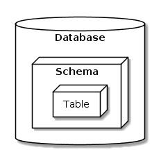
Our database is divided into a few “schemas” – if our database is a big filing cabinet, we can imagine the schemas as separate drawers. You can see all of them using the ojo_list_schemas() function.

library(ojodb)
library(dplyr)

ojo_list_schemas()
#> # A tibble: 9 × 1
#>   schema            
#>   <chr>             
#> 1 archive           
#> 2 doc_tracker       
#> 3 eviction_addresses
#> 4 eviction_dashboard
#> 5 iic               
#> 6 ocdc              
#> 7 odoc              
#> 8 oscn              
#> 9 public

Each schema, generally speaking, relates to one of our data types / topics / policy areas. Each one contains tables that store data related to that policy area. Among others, we have:

a schema for ocdc (Oklahoma County Detention Center, i.e. the jail in Oklahoma City),
another one for odoc (Oklahoma Department of Corrections, i.e. Oklahoma state prisons),
another for eviction_addresses (this one contains data related to a specific eviction-related project)

A diagram I found online that shows how our database is structured.

The court data that we’re interested in right now is stored in the default schema, public. Let’s open the “drawer” and see what kind of data is inside.

ojo_list_tables(schema = "public")
#> # A tibble: 18 × 2
#>    schema table           
#>    <chr>  <chr>           
#>  1 public address         
#>  2 public appellate_count 
#>  3 public attorney        
#>  4 public attorney_address
#>  5 public case            
#>  6 public case_type       
#>  7 public citation        
#>  8 public count           
#>  9 public event           
#> 10 public exception_log   
#> 11 public issue           
#> 12 public marital_status  
#> 13 public migrations      
#> 14 public minute          
#> 15 public party           
#> 16 public person_record   
#> 17 public process_log     
#> 18 public representation

If a schema is a drawer in our filing cabinet, then tables are the folders inside. The public schema contains several different tables, all of which relate back to our court data. Here are the most important ones to know:

The case table contains the basic information about each case. This includes variables like the case number, the date it was filed, the judge it was assigned to, etc. It also includes ID columns that allow you to join it with the other tables in this schema in order to see things like the defendant’s name and DOB, attorneys involved, etc. Each row is one case.
The count table contains the individual charges filed in each case; most cases involve more than one. Each row is one charge.
The minute table contains the court minutes for each case. This is where we get data about court fines and fees, among many other things. There are a ton of minutes per case, so working with the minute data often means having to spend a lot of time waiting for data to download. Each row is one court minute.

We can see exactly which variables are included in each table using the ojo_list_vars() function. For example, let’s take a closer look at the main case table:

ojo_list_vars(schema = "public", table = "case")
#> # A tibble: 21 × 1
#>    column_name         
#>    <chr>               
#>  1 appealed_from       
#>  2 attorneys           
#>  3 case_number         
#>  4 case_type           
#>  5 citation_information
#>  6 counts              
#>  7 created_at          
#>  8 date_closed         
#>  9 date_filed          
#> 10 district            
#> # ℹ 11 more rows
#> # ℹ Use `print(n = ...)` to see more rows

We’re interested in criminal cases right now, so we’ll be pulling data from this table for our example research question.

Step 2: Pulling our data – `ojo_crim_cases()`

Now that we understand the basic layout of the database, we can start pulling the data we’re interested in! Fortunately, we have helper functions that save us from having to think too much about schemas and tables in our daily work.

Keeping our research question in mind, we’ll start by pulling all the misdemeanor criminal cases filed in Oklahoma and Tulsa counties from 2016-2022. We’ll use one of our helper functions, ojo_crim_cases(), to do so. It first queries the case table, then combines that table of cases with each case’s charges from the count table.

# This function combines the "case" and "count" tables in our database,
# and returns a cleaned dataframe where each row is one charge in a case.
charge_data <- ojo_crim_cases(districts = c("OKLAHOMA", "TULSA"),
                              case_types = "CM", # "CM" is short for "criminal misdemeanor"
                              file_years = 2016:2022) |>
  # you can add things like filter(), select(), etc. here
  collect()

The collect() function we’re using is from the dplyr package. Our helper function ojo_crim_cases() uses the provided arguments to put together a query to our database, and the collect() function executes that query and returns the result as a lazy tibble into your R environment. If we wanted to, we could add in additional filtering, sorting, etc. by adding dplyr functions like filter(), select(), etc. before the collect() call. But for now, we want to see everything.

Exploring the data we’ve pulled

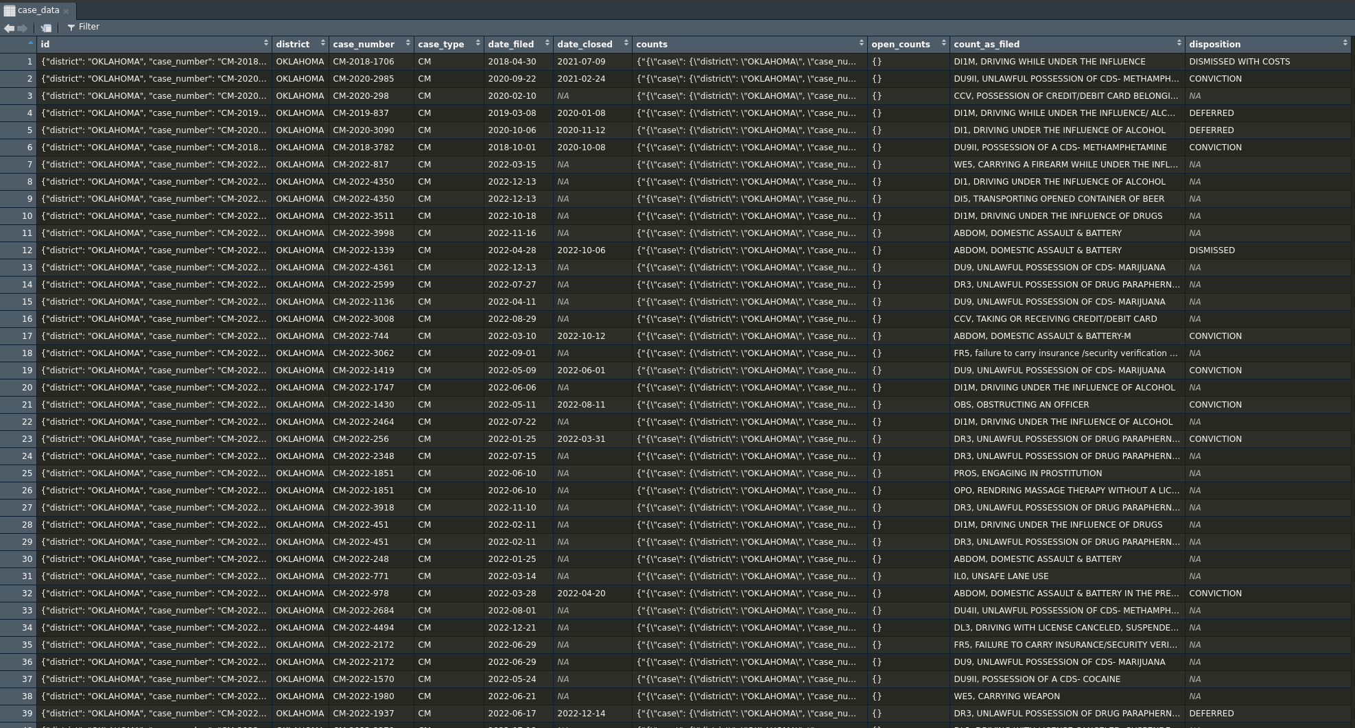
Now we’ve got our data saved as the object charge_data, nice! Before we do anything else, let’s start by taking a look at our dataframe in RStudio using the View() function (or just by clicking on it in your RStudio “Data” panel).

The result of View(charge_data)

Charges vs. Cases?

You’ll probably notice that our dataframe includes data on the individual charges in each case, stored in count_as_filed and disposition. As discussed above, there’s often going to be more than one charge involved in a given case, which means that we should note that our data is in terms of charges, not cases. Let’s start by seeing how many of each we have here:

# How many total charges? ------------------------------------------------------
# The data are already in terms of charges (1 charge per row), so we can simply
# count the rows.
charge_data |>
  nrow()
#> [1] 111205

# How many total cases? --------------------------------------------------------
# There's more than one charge per case sometimes, so we need to see how many
# unique cases there are total. Here are two possible approaches:

# Approach #1: Creating a new, unique district + case_number variable
charge_data |>
  # Case numbers are unique within districts; 
  # e.g. Tulsa's CM-2023-001 is a different case than Oklahoma's CM-2023-001.
  # We can create a new variable that will always be unique -- district + case_number
  mutate(case_number_with_district = paste(district, case_number)) |>
  distinct(case_number_with_district) |>
  nrow()
#> [1] 62187

# This approach returns the number of unique case_number / district combinations, 
# but not much else.

# Approach 2: Making a new summary dataset with group_by() + summarize()
case_summary <- charge_data |>
  group_by(district, case_number) |>
  summarize(
    n_charges = n()
    # Note: if you want, you can add further summary variables here. 
    # For example, maybe you want to know how many charges in each case led to
    # a conviction. You could do something like this:
    # n_convictions = sum(disposition == "CONVICTION", na.rm = T)
  )

nrow(case_summary)
#> [1] 62187

# This tells us the number, and also leaves us with a helpful new case_summary
# dataset that we can use later on, if we want to know more.

It looks like charge_data includes 111,205 rows. In other words, our data shows that there were 111,205 total charges filed in Oklahoma and Tulsa county misdemeanor cases from 2016-2022.

On the other hand, it looks like there are 62,187 unique combinations of district and case_number (and an equal number of rows in our new summary dataframe, case_summary). In other words, our data shows 62,187 total misdemeanor cases filed in Oklahoma and Tulsa county from 2016-2022.

If we wanted to, we could divide those numbers (or use our handy case_summary dataframe) to see the average number of charges per case:

# Total charges / total cases = Avg. number of charges per case
nrow(charge_data) / nrow(case_summary)
#> [1] 1.788235

# Different approach, same thing
mean(case_summary$n_charges)
#> [1] 1.788235

It seems there’s an average of 1.79 counts per misdemeanor case in this dataset. Neat!

It’s very helpful to always be thinking about what the rows in your data represent. Keeping track of what exactly you’re looking at (charges, cases, defendants, etc.) can be one of the most challenging parts of these analyses, especially when our client isn’t exactly sure which they want to know about.

Did we get everything we asked for?

Though we have data coverage and quality checks already as part of our scrapers and database, court data is always extremely messy, which can lead to unforeseen issues. Knowing this, it’s usually a good idea to double check your data after you’ve pulled it in order to ensure ojo_crim_cases() returned all the data you requested.

We should at least check the data geographically and temporally; in other words, we should make sure there aren’t any weird, unexpected differences between counties or between filing years / months. How exactly you do this due diligence is up to you, but one potential approach is to make a quick visualization or two. For example:

library(lubridate)
library(ggplot2)

# We're going to look at charges, not cases here
charge_data |>
  mutate(
    # Our end goal is to see monthly filings, so we'll use that same timeframe
    month_filed = floor_date(date_filed, "months")
  ) |>
  count(district, month_filed) |> # Our two most important checks, geography and time
  ggplot(aes(x = month_filed,
             y = n)) +
  # I'm choosing geom_col() over geom_line() because I want to see any gaps clearly
  geom_col() + 
  facet_wrap(~district) +
  scale_y_continuous(limits = c(0, NA)) +
  labs(title = "Total charges filed per month in CM cases")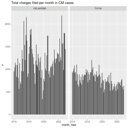

This graph looks pretty much as we’d expect it to – there’s not a huge difference between Oklahoma and Tulsa counties (which makes sense, given that they’re similar in size), and there aren’t any conspicuously missing months, suspiciously massive and sudden spikes / drops, etc. And while there is a lot of variation (particularly in Oklahoma county), there’s nothing that looks suspicious enough for me to suspect a data issue.

It would be great if there was an absolute source of truth that we could use to double check this stuff more reliably. An internal data quality monitoring dashboard that serves this purpose is on our list of goals, and hopefully that will serve as an easy reference point in the future. But for now, this part of the process is all about looking at the data from different angles and thinking critically about where you might run into potential issues, and how those issues might show up in your testing. Referencing past OKPI work is also another good option, and so is asking another analyst who is more familiar with the data in that area.

Back to our research question

Now we’ve got a big dataset of all the charges we care about (charge_data) and another big dataset of all the cases we care about (case_summary), we’ve familiarized ourselves with what they look like and what they mean, and we’ve double checked that the data are all there. Let’s revisit our research question now to see what cleaning and wrangling we need to do in order to finish answering it.

How many misdemeanor cases involving drugs were filed in Oklahoma and Tulsa county in each month from 2016-2022?

We’ve got the “misdemeanor cases filed in Oklahoma and Tulsa county from 2016-2022” part down, but we’re still missing a few things. Namely,

we still need to filter our data to include only cases involving drugs, and
we still need to calculate the number of cases filed per month in this timespan.

We’ll move on to those steps next.

Step 3: Wrangling, cleaning, and analyzing the data

First, we’ll need to limit our dataset to cases involving drugs. But what exactly does that mean? Do we want any kind of case at all where at least one of the charges was drug-related, or only cases where all the charges were drug related? What exactly do we count as “drug-related” charges, anyway? Frequently, our partners will make vague asks like this and leave it to us to answer those questions.

You’ll also notice that the data in the count_as_filed column is very messy, and we won’t be able to do something as simple as filter(count_as_filed == "Drug Possession"). So we’ll need to find a way of parsing that text in order to find the charges we need.

The answers to these methodology questions will depend on the exact task at hand, but our goal is to make our research methodology as standardized and replicable as possible. That also means we don’t want to re-invent the wheel – Open Justice Oklahoma has done lots of work on drug laws in the past, and so we have a fairly well established way of searching the statutes for relevant charges. Here are some of the places you can go to see how OJO has handled methodology / data issues in the past:

The Oklahoma Policy Institute Stack Overflow site has a Q/A format like the Stack Overflow we all know and love. If you run into a new issue we don’t have documented here, feel free to add your own questions / answers as needed!
Searching the Open Justice Oklahoma Github repos for keywords can sometimes turn up past work, especially when you’re dealing with a more technical coding issue.
The Oklahoma Policy Institute blog page has finished products we’ve helped put out in the past, with work on evictions, drug laws, felony reclassification, fines and fees, etc.
And, of course, please don’t hesitate to ask on Slack! It’s easy for things to get lost in the shuffle and not make it into documentation anywhere, and despite our efforts, there are still a lot of things that only live inside someone’s brain.

In this case, we’re going to use a regex string that OJO’s founder Ryan Gentzler originally wrote to find any kind of drug-related charge, including things like paraphernalia, trafficking, etc. Here’s the string:

drugs <- "CDS|C\\.D\\.S|DRUG|OXY|HUFF|AMPHET|ZOLOL|ZOLAM|HYDROC|CODEIN|PRECURS|
|XANAX|MORPH|METERDI|ZEPAM|LORAZ|VALIU|EPHED|SUB|COCA|PSEUDO| CD|CD |PRESCRIP|
|NARC|METH|C\\.D\\.|HEROIN|ANHYD|AMMONIA|OPIUM|LORTAB|MARIJUANA|CANNABIS|MJ"

While I was writing this vignette, I found it by searching “drugs” and “marijuana” on our Github. It should really be a lot easier and more streamlined than that, though, so in the future this will hopefully be integrated as part of the ojodb package.

We’ll start by adding a new variable that simply classifies each charge as drug-related or not.

# We'll save it as a new dataframe, charge_data_cleaned
charge_data_cleaned <- charge_data |>
  select(-c(id, counts, open_counts)) |> # We don't need every column, so let's drop the extras
  mutate(
    drug_charge = grepl(pattern = drugs, # Do any of our "drug" strings...
                        x = count_as_filed, # ...show up in count_as_filed?
                        ignore.case = TRUE) # ignore.case is important!
  )

Note the inclusion of ignore.case = TRUE! Although most of the data in the count_as_filed column is in uppercase, you shouldn’t assume anything in this court data will be uniform. Much of it is hand-entered by the county clerks, and there are frequent typos, differences in phrasing between districts, random lowercase entries, etc. It is very messy, which means we have to be vigilant when it comes to double-checking our work and not making too many assumptions about the data.

Again, let’s stop and check to make sure the result looks as we expect it to.

charge_data_cleaned |>
  select(district, case_number, count_as_filed, drug_charge) |>
  group_by(drug_charge) |>
  slice_sample(n = 10) # We'll just look at a random sample of 10 in each category
#> # A tibble: 20 × 4
#> # Groups:   drug_charge [2]
#>    district case_number  count_as_filed                              drug_charge
#>    <chr>    <chr>        <chr>                                       <lgl>      
#>  1 TULSA    CM-2020-1563 VPO, VIOLATION OF PROTECTIVE ORDER          FALSE      
#>  2 OKLAHOMA CM-2022-248  ABDOM, DOMESTIC ASSAULT & BATTERY           FALSE      
#>  3 TULSA    CM-2017-628  RR4, DRIVING W/O DRIVER'S LICENSE ON PERSON FALSE      
#>  4 OKLAHOMA CM-2017-3105 DI1, DRIVING WHILE UNDER THE INFLUENCE      FALSE      
#>  5 TULSA    CM-2017-4789 LC3, DRIVING LEFT OF CENTER                 FALSE      
#>  6 OKLAHOMA CM-2021-1747 DL7, DRIVING WITHOUT A DRIVER'S LICENSE     FALSE      
#>  7 TULSA    CM-2016-5514 EDUC, VIOLATION OF COMPULSORY EDUCATION ACT FALSE      
#>  8 TULSA    CM-2017-5360 ST1, FAIL TO STOP FOR STOP SIGN             FALSE      
#>  9 OKLAHOMA CM-2019-2012 CDEL, CONTRIBUTING TO THE DELIQUENCY OF A … FALSE      
#> 10 OKLAHOMA CM-2021-3436 DL3, DRIVING WITH LICENSE CANCELED, SUSEPN… FALSE      
#> 11 TULSA    CM-2020-1218 DI2DM, DRIVING UNDER THE INFLUENCE OF DRUGS TRUE       
#> 12 OKLAHOMA CM-2018-1507 DR3, POSSESSION OF DRUG PARAPHERNALIA       TRUE       
#> 13 OKLAHOMA CM-2021-1125 DI1, DRIVING UNDER THE INFLUENCE OF DRUGS   TRUE       
#> 14 TULSA    CM-2019-3346 DU9II, POSSESSION OF CONTROLLED DRUG METHA… TRUE       
#> 15 OKLAHOMA CM-2019-986  DR3, POSSESSION OF DRUG PARAPHERNALIA       TRUE       
#> 16 TULSA    CM-2020-4341 DU4III, UNLAWFUL POSSESSION OF CONTROLLED … TRUE       
#> 17 TULSA    CM-2022-2668 DI2, DRIVING UNDER THE INFLUENCE OF DRUGS … TRUE       
#> 18 OKLAHOMA CM-2021-1256 DI1, DRIVING UNDER THE INFLUENCE OF DRUGS … TRUE       
#> 19 TULSA    CM-2016-1387 DR3MV, POSSESSION OF DRUG PARAPHERNALIA     TRUE       
#> 20 TULSA    CM-2018-744  TU0, REQUIRED POSITION & METHOD OF TURNING  TRUE

It looks like our regex search was pretty successful! Although it may raise some new questions: does driving under the influence count? Is alcohol technically a “drug” in those cases, or is that different? What about a count description that says “Carrying a firearm while under the influence o drugs or alcohol”?

There are always going to be more questions like this, and you’ll find them when you start digging in and double-checking your data. In the end, we want to prioritize standardization and giving our client whatever they actually want / need (even if we have to help them figure out exactly what that is). For now, we’ll just accept the result as-is, but at this point you might need to stop, re-assess some things, ask other analysts / policy team their thoughts, follow up with a client, etc.

Summarizing drug charges within cases

We have one more wrangling task we need to figure out – we know what counts as a drug charge, but what about a drug case? For our purposes, we’ll say that a drug case means any case involving at least one drug charge. Therefore, we’re going to make another version of our case_summary dataframe, this time with a new variable drug_charges_present:

case_summary_cleaned <- charge_data_cleaned |>
  group_by(district, case_number) |>
  # We want to keep the date_filed, so we'll use transmute() this time instead of summarize()
  transmute( 
    date_filed = date_filed,
    # It will be helpful to have all the values of count_as_filed verbatim for double-checking
    list_all_charges = paste(count_as_filed, collapse = "; "),
    n_total_charges = n(),
    # Count the number of rows where drug_charge == TRUE
    n_drug_charges = sum(drug_charge, na.rm = TRUE),
    drug_charges_present = if_else(n_drug_charges > 0, TRUE, FALSE)
  ) |>
  ungroup() |>
  distinct() # transmute() leaves duplicate rows, so we'll drop those

# Alternative approach:
# case_summary_cleaned <- charge_data_cleaned |>
#   group_by(district, case_number) |>
#   summarize( 
#     date_filed = unique(date_filed),
#     list_all_charges = paste(count_as_filed, collapse = "; "),
#     n_total_charges = n(),
#     n_drug_charges = sum(drug_charge, na.rm = TRUE),
#     drug_charges_present = if_else(n_drug_charges > 0, TRUE, FALSE)
#   ) |>
#   ungroup()

We’ll also save a new dataframe that only includes the drug cases. We can double check the result just like before, and see how many drug cases we have total:

case_summary_cleaned_drugs <- case_summary_cleaned |>
  filter(drug_charges_present)

case_summary_cleaned |>
  group_by(drug_charges_present) |>
  slice_sample(n = 10)
#> # A tibble: 20 × 7
#> # Groups:   drug_charges_present [2]
#>    district case_number  date_filed list_all_charges             n_total_charges
#>    <chr>    <chr>        <date>     <chr>                                  <int>
#>  1 TULSA    CM-2019-5335 2019-11-20 DI1M, DUI ALCOHOL (MUNICIPA…               1
#>  2 TULSA    CM-2018-3174 2018-07-24 DI1M, DUI ALCOHOL (MUNICIPA…               1
#>  3 OKLAHOMA CM-2017-1221 2017-04-24 DI3, DRIVING WHILE UNDER TH…               1
#>  4 TULSA    CM-2017-1707 2017-04-18 PUBSFT, INTERFERING WITH FI…               1
#>  5 OKLAHOMA CM-2016-1403 2016-05-23 VPO, VIOLATION OF PROTECTIV…               1
#>  6 OKLAHOMA CM-2020-2887 2020-09-10 OBS, OBSTRUCTING AN OFFICER…               2
#>  7 TULSA    CM-2022-1865 2022-06-03 EMB, EMBEZZLEMENT UNDER $500               1
#>  8 TULSA    CM-2016-5403 2016-10-27 ABDOM, ASSAULT AND BATTERY …               2
#>  9 OKLAHOMA CM-2020-2652 2020-08-19 DI1AG, AGGRAVATED DRIVING U…               1
#> 10 TULSA    CM-2021-1634 2021-05-05 WE5, UNLAWFULLY CARRYING A …               1
#> 11 TULSA    CM-2018-2288 2018-05-31 DU9II, UNLAWFUL POSSESSION …               3
#> 12 TULSA    CM-2017-2639 2017-06-13 FR5, FAILURE TO CARRY INSUR…               4
#> 13 TULSA    CM-2017-4969 2017-10-27 DU9IV, POSSESSION OF CONTRO…               2
#> 14 OKLAHOMA CM-2017-2558 2017-07-28 DU9II, POSSESSION OF A CDS …               2
#> 15 TULSA    CM-2017-4171 2017-09-14 DU9, POSSESSION OF CONTROLL…               1
#> 16 TULSA    CM-2018-2149 2018-05-21 DU9, POSSESSION OF CONTROLL…               1
#> 17 TULSA    CM-2017-3494 2017-08-03 DU9II, UNLAWFUL POSSESSION …               2
#> 18 TULSA    CM-2022-2693 2022-08-11 DI1M, DRIVING UNDER THE INF…               4
#> 19 TULSA    CM-2020-3164 2020-09-17 IL1, UNSAFE LANE USE; S21, …               4
#> 20 TULSA    CM-2022-3608 2022-10-25 FR5, FAILURE TO CARRY INSUR…               5
#> # ℹ 2 more variables: n_drug_charges <int>, drug_charges_present <lgl>

# view(case_summary_cleaned)

# What proportion of these CM cases feature a drug charge?
nrow(case_summary_cleaned_drugs) / nrow(case_summary_cleaned)
#> [1] 0.2604724

Nice! Now we have some nice, clean datasets to visualize. This stage of analysis is tough sometimes; it involves a lot of subjective decision-making, a lot of making the most of messy data, and a lot of double-checking of work. But even though we’re aiming for standardized methods, it’s also one of the areas where we get to exercise a little bit of creativity and come up with our own solutions to things, so feel free to blaze your own path a little bit too!

Step 4: Visualizing and exporting the data

To finish things off, we’re going to make ourselves a nice, pretty graph showing how many of our drug cases were filed each month throughout the timespan of our data. We’ll be using the ojo_theme() and ojo_colors() functions from ojodb to take care of most of the styling.

case_summary_cleaned_drugs |>
  mutate(
    month_filed = floor_date(date_filed, "months")
  ) |>
  count(month_filed, district) |>
  ggplot(aes(x = month_filed,
             y = n,
             color = district)) +
  geom_line() +
  scale_y_continuous(limits = c(0, NA)) + # Usually we want to show the y-axis down to zero
  ojo_theme() +
  ojo_color() +
  labs(
    title = "CM cases involving at least one drug charge,",
    subtitle = "Oklahoma and Tulsa county district courts, 2016-2022",
    x = "Month of case filing",
    y = "Total drug cases filed",
    caption = "Source: Open Justice Oklahoma analysis
    of Oklahoma State Court Network (OSCN.net) data.",
    color = "District"
  )

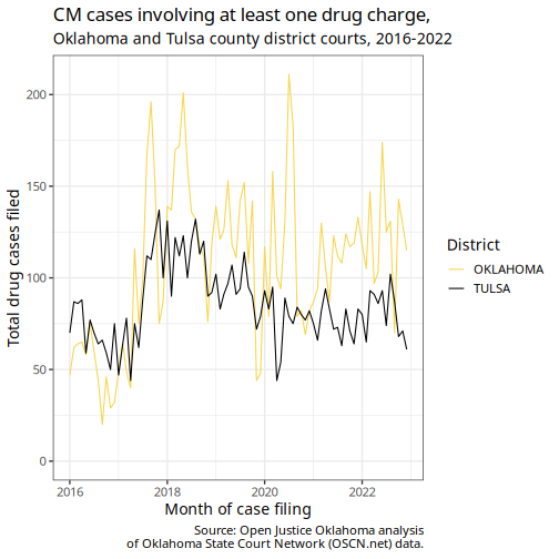
Looking good! If you’re curious about the increase seen around July of 2017, you can read about why that happened here.

We also frequently need to send out data in spreadsheet form. You’ll typically want to export datasets using the readr package in whatever format your client needs. A good default option is our old friend the Comma Separated Values format, .csv. Here, we’d do that with write_csv(case_summary_cleaned_drugs, "export-data.csv"). Exporting to the Microsoft Excel spreadsheet format .xlsx will require the readxl package.

Step 5: Review and deliver

The last step in the process is to submit your work for a review. Ideally, we should try to make sure everything we do has at least two people (an analyst and a reviewer) look over it before we send it out to a client or publish it. The review process should check every step in the process, and include any needed discussions about the methodological questions we talked about earlier.

We’re aiming to start doing reviews via Github. The process will essentially be:

Open a pull request with all your code.
Request a reviewer on the pull request, and let them know you’re ready for them to look it over via Slack, etc.
They should pull your code from GitHub and run it locally on their machine, checking each step of the process along the way. Any notes, changes, etc. should be included in their review on GitHub, so you can see everything in one convenient place.
Once all edits have been addressed, we can merge the pull request and we’ll have a nice finished product on our main branch!

From there, all you’ll have to do is write up an email (or whatever delivery method is relevant) and send your data / visualizations out to whoever needs them.

If I wrote all of this correctly and you managed to follow along, then congratulations to both of us! You’ve successfully learned how to pull court data from the OJO database and use it to answer a research question about our legal system. You’ll probably run into a lot of things that aren’t covered in this vignette as you tackle new questions and use new parts of our data, but hopefully this will be a useful resource as you’re starting out.

Just remember – the data is very quirky, and there’s always going to be stuff you don’t know and problems you aren’t sure how to solve. Whether it’s a methodology issue, a coding issue, a “dealing with a client” kind of issue, whenever you find yourself spinning your wheels, please don’t hesitate to just ask! There’s a good chance OJO has been there before, and if not, we’ll figure it out together. Thanks for reading!